There are moments in research where you suddenly have an euphoric rush once you truly understand the beauty of something. First such moment happened to me when I got the beauty of SU(2) spinor group. Couple of days ago, I had the same cathartic moment when I finally got the brilliance of BdG Hamiltonians. This post is just to clarify to my future self if I get stuck understanding this again. In this first post, let me outline the basic super conductive nature with a simple 2 site system.
So, Lets try to understand a rudimentary superconductor that is made up of 2 sites ($a,b$) with no hopping between them. The Hameltonian can be written as
\[\mathcal{H}=E_ac^\dagger_ac_a+E_bc^\dagger_bc_b+\Delta c^\dagger_a c^\dagger_b +\Delta^* c_b c_a \label{eq:1}\]First part with $E_a$ and $E_b$ terms are the cost for the electron to stay in each site whole $\Delta$ is the superconducting pairing term that pairs the electron creating or destroying them in both sites. This term forces us to forgo our faithful single particle basis to represent the Hamiltonian, as one can clearly see that $\mathcal{H}$ involves two particle term. So, as would a many body theorist do, lets solve it in the two particle basis.
\[\mathcal{H}=\begin{bmatrix} E_a & 0 & 0 & 0\\ 0 & E_b & 0 & 0\\ 0 & 0 & E_a+E_b &\Delta \\ 0& 0 &\Delta^* &0 \end{bmatrix}\label{eq:2}\]The basis order chosen is ($\vert a,0 \rangle,\vert a,b \rangle,\vert a,b \rangle,\vert 0,0 \rangle$). Because of the block diagonal nature of H, it is clear to see that two of the Eigen values are $E_a,E_b$. It would be easy to solve $H$ analytically as its just 4x4 matrix. But instead, let us solve it numerically just for fun.
We start by defining the matrix in python given by
import numpy as np
import matplotlib.pyplot as plt

def H_bdg(e1=0,e2=1,d=1,eig=True):
    H=np.array([
                [e1,0,0,0],
                [0,e2,0,0],
                [0,0,e1+e2,d],
                [0,0,np.conj(d),0]
    ])
    if eig:
        eig1,eval=np.linalg.eig(H)
        return eig1,eval
    else:
        return H

eig,eval=H_bdg()
for i,j in zip(eval,eig):
    print("eig: ",np.round(j,3),"\t E vec: ",np.round(i,3))

fig,ax=plt.subplots(figsize=(2,4))
for i in eig:plt.axhline(i,c="k",lw=4)
plt.ylabel("Energy")
plt.tight_layout()
plt.show()
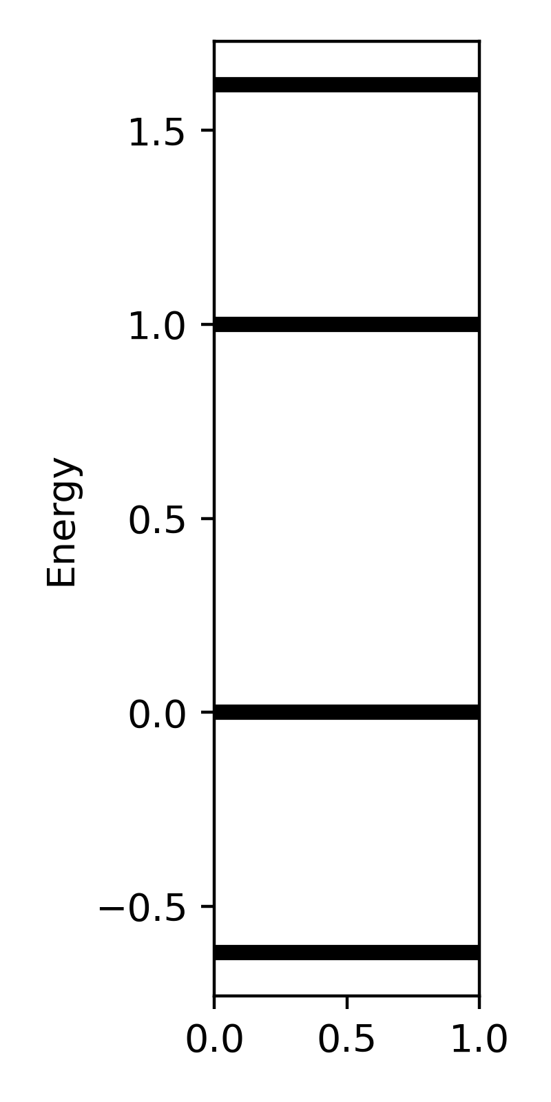
For the test, we choose $E_a=0,E_b=1,\Delta=1$. Now plotting the eigen value, we get

We see that we have two eigen values at 0 and 1 as we choose $E_{a,b}$ to be that and then there are other eigen value that belong to the two particle subspace. Well this is where things get interesting. Its exactly this fact that we are going to exploit to understand the system - that we can split the Hamiltonian into blocks of single and two particle. A block diagonal form means, we have a symmetry in our system, and that symmetry is nothing but Parity. This is the symmetry that our eigen vectors can now be labeled by a number which specifies if it belongs to the single particle block or the two particle block. To this end, let us construct the parity operator.
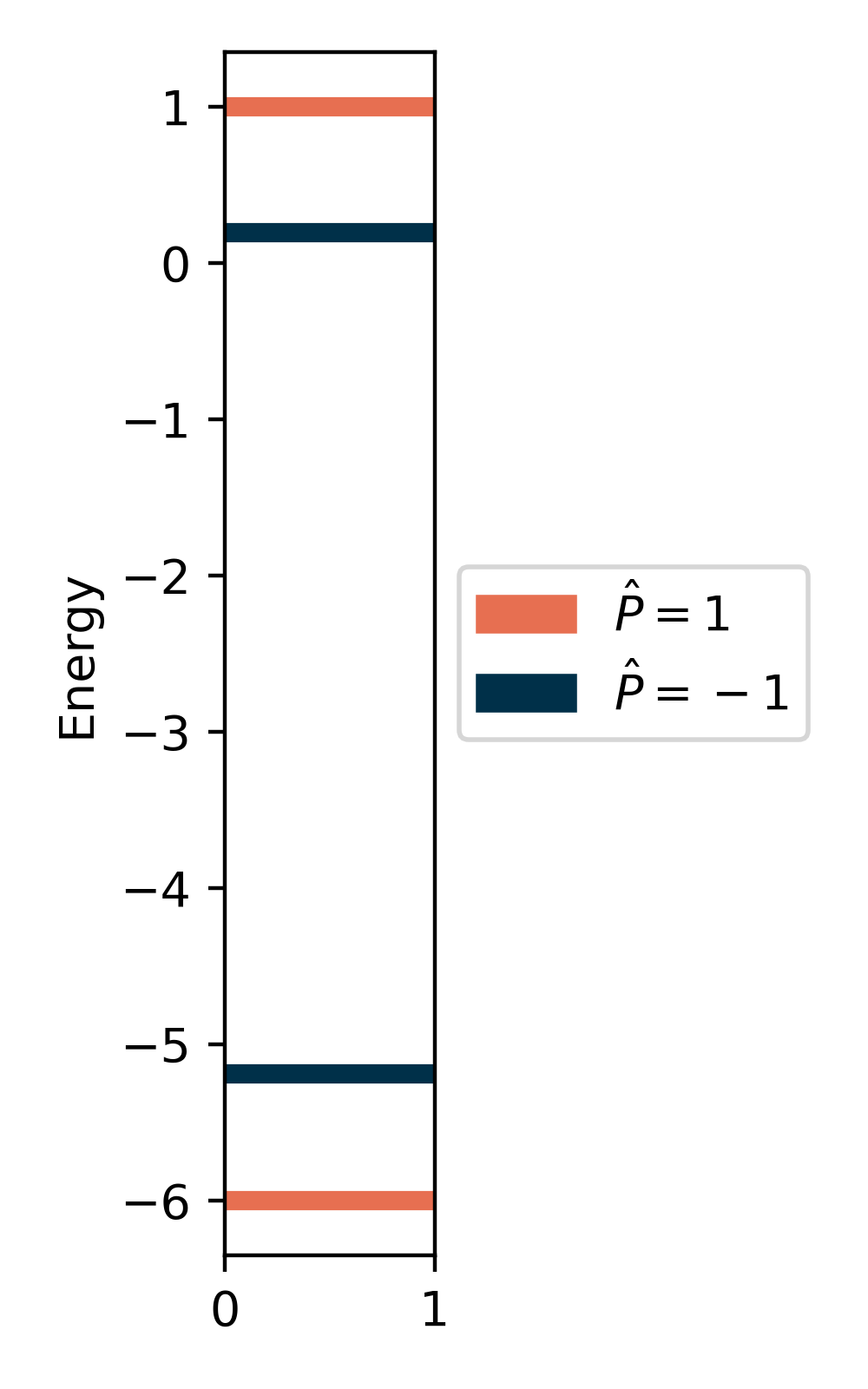
\[\hat{P}=\begin{bmatrix} 1 & 0 & 0 & 0\\ 0 & 1& 0 & 0\\ 0 & 0 & -1 &0 \\ 0& 0 &0 &-1 \end{bmatrix}\label{eq:3}\]It is easy to see that $PP^\dagger=0$ this operator when acted on our basis, spits either 1 or -1 based on if the eigen value is in single particle or multi particle subspace. Now let us color our eigen value based on this operators expectation value.
P=np.array([
    [1,0,0,0],
    [0,1,0,0],
    [0,0,-1,0],
    [0,0,0,-1]
])
c=[np.round(eval[n]@P@eval[n].conj()) for n in range(4)]
fig,ax=plt.subplots(figsize=(2.5,4))
for j in range(4):plt.axhline(eig[j],c="r" if c[j] ==1 else "b",lw=4)

import matplotlib.patches as mpatches
red_patch = mpatches.Patch(color='red', label='$\hat{P}=1$')
blue_patch = mpatches.Patch(color='blue', label='$\hat{P}=-1$')

plt.legend(handles=[red_patch, blue_patch],loc="center left",bbox_to_anchor=(1,0.5))

plt.ylabel("Energy")
plt.tight_layout()
plt.savefig("Manybody_eigen_colered.png",dpi=400)
plt.show()
This gives us the following plot

As you can see, the lowest energy ground state of the system is made up of two particle ground state while the first excited state is made up of single particle state. Parity here says if we have any unpaired electron in our system or if all the electrons are paired. Now we can study this system as a function of a parameter,

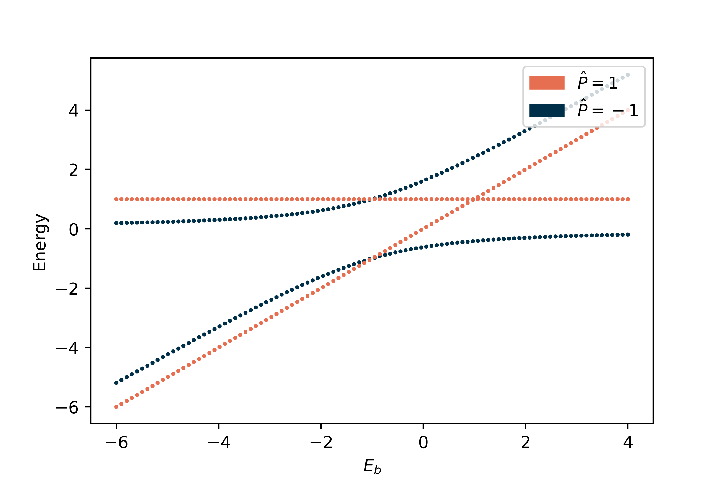
Here, we plot the eigen values projected on the parity subspace as a function of $E_b$ for $E_a=1,\Delta=1$. Here is the beauty, the ground state of this system after around $E_b>-1$ switches in parity and thus starts having one unpaired electron that has a finite energy gap to be paired. This thus gives amazing physical result as superconductivity.
We will look at how this entire discussion can be mapped in BdG formalism in the next post …
Topics to explore
physics coding topology python perovskite numba Monte-carlo Julia tight-binding talk susceptibility spin-waves quantum quamtum pysktb optimization finance field-theory advisor Superconductivity Slaster-koster Quantum QFT Physics BdG