So here is the deal, I have been trying to convince my professor that we should start implementing our new codes (which solves not so super heavy equations with 4-point feynman diagrams) in python than FORTRAN. This is done mostly because, I am more fluent in python and also at some point I want to port it to Julia, the new kid in the block. I have known about numba for sometime and had wanted to try it, so what better way than to introduce the idea of emergence using numba to prove a point !
Okay, Lets start by saying our goal is to make a rudimentary model to understand the crowd mentality in stock market i.e. how the market as a whole reacts to negative or positive news.
Say the market is made up \(n \times n=n^{2}\) of people with everyone living in a hypothetical flat land who trade a particular sector (like financial sector or tech stocks). In this world, everyone is in a state of “buy” or “sell” which we will take it to be \(+1\) or \(-1\). Thus the measure that market tries to minimize is given by
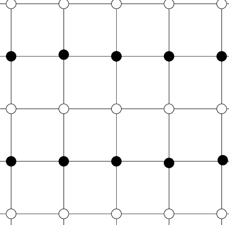
\[\begin{equation}\hat{H}=J\sum_{i,j}\hat{\sigma_i} \hat{\sigma_j}\end{equation}\]First we will describe what the variables mean and then see why market would try to minimize this. Here \(\hat{\sigma_i}\) is the state operator, meaning given a state of market it would pick the sentiment of \(i^{th}\) person. For example, lets say the market is made up of 4 people (extremely small world, but meh!), then the state of the market, say is \(|s>=(1,1,-1,1)\) meaning the first and second person wants to buy (\(1,1\)) are the first two elements, while the third and fourth one wants to sell denoted by (\(-1,-1\)) which are the last two elements. Then \(\hat{\sigma_2}|s>=1\) just picks the second person’s sentiment. \(J\) here defines the influence of our nearby trader circle (for example listening to a podcast about stock market might influence your sentiment and hence everyone who listens to the podcast would be influenced the same way). Now we need a final ingredient which we will call randomness \(R\) which influences randomness in our market. This is essentially controls how our group’s sector is not self contained, meaning our traders often get influenced by what happens in other sectors too. For example, what happens to utility sector is strongly influenced by real-estate markets. But since we are just modeling one sector, we will include this effect as a randomness \(R\). Finally the sum in \(H\) is with nearest neighbor i.e. person close to each other. How do we know who is close to who? well thats where our approximation of flat land comes into play, we will put our investors in a 2 dimensional square grid and hence each person would be surrounded by 4 person next to each other as shown where each black dot is connected to 4 nearest white dots

To see how \(H\) signifies a market, what we have said in \(H\) is that whenever we are same or different from our neighbors, we pay a cost of \(|J|\) and thus the market as an entirety tries to pay the lowest cost.
Now we are ready to study this system. This is what we are going to do. We will start with a initial configuration of market that is generated by random and calculate what \(H\) is and then switch the sentiment of some one in random and see if it reduces the cost. If it does, we will take that as the new normalcy of market. If it doesn’t reduce the cost, we will still accept it with a probability of \(e^{-R \Delta H}\) where \(\Delta H\) is the cost of changing the sentiment of that one person. Thus as time proceeds, we will see what happens to the total market sentiment.
To code this, we will first import all required python libraries
%matplotlib inline
import numpy as np
from numpy.random import rand
import matplotlib.pyplot as plt
import numba as nb
from numba import jitclass
import matplotlib.pyplot as plt
import matplotlib.gridspec as gridspec
Then without going into details (which is quite straight forward) we have the following code that calculates the total sentiment of the market as time proceeds
def initialstate(N):
    state = 2*np.random.randint(2, size=(N,N))-1
    return state

@nb.jit(nopython=True)
def mcmove(config, beta,N,J=1):
    for i in range(N):
        for j in range(N):
                a = np.random.randint(0, N)
                b = np.random.randint(0, N)
                s =  config[a, b]
                nb_1 = config[(a+1)%N,b] + config[a,(b+1)%N] + config[(a-1)%N,b] + config[a,(b-1)%N]
                cost = 2*J*s*nb_1
                if cost < 0:
                    s *= -1
                elif rand() < np.exp(-cost*beta):
                    s *= -1
                config[a, b] = s
    return config
@nb.jit(nopython=True)
def calcEnergy(config,N,J=1):
    energy = 0
    for i in range(len(config)):
        for j in range(len(config)):
            S = config[i,j]
            nb_1 = config[(i+1)%N, j] + config[i,(j+1)%N] + config[(i-1)%N, j] + config[i,(j-1)%N]
            energy += -nb_1*S
    return energy/4.
@nb.jit(nopython=True)
def calcMag(config):
    mag = np.sum(config)
    return mag
def calculate(T=2.3,N= 16,eqSteps = 1024,mcSteps = 1024,state=0,J=1):
    E=np.zeros(mcSteps)
    n1, n2  = 1.0/(mcSteps*N*N), 1.0/(mcSteps*mcSteps*N*N)
    E1 = M1 = E2 = M2 = 0
    config = initialstate(N)
    iT=1.0/T; iT2=iT*iT;

    for i in range(eqSteps):
        mcmove(config, iT,N,J)

    for i in range(mcSteps):
        mcmove(config, iT,N,J)
        E[i]=calcMag(config)
    return E
and then plot it using
J=1
T=np.linspace(2.3,2.8,4)
fig,ax1 = plt.subplots(2,2,figsize=(15,8))
plt.rcParams.update({'font.size': 12})
i1=0;j1=0
for i,j in enumerate(T):
    n=4000
    ax=ax1[i1][j1]
    j1+=1
    if j1==2:i1+=1;j1=0
    E=calculate(T=j,N=36,eqSteps=1,mcSteps=n,J=J)/n
    #plt.plot(range(len(E)),E,c="k",ls=":",alpha=.2)
    ax.fill_between(np.arange(len(E)),E,where=E>0.,interpolate=True,color="g")
    ax.fill_between(np.arange(len(E)),E,where=E<0.,interpolate=True,color="r")
    ax.set_xlabel("time")
    ax.set_ylabel("Sentiment")
    ax.set_title("J={}  R={}".format(J,np.round(j,2)))
plt.tight_layout()
plt.savefig("JvsR1.png",dpi=400)
plt.show()
giving us

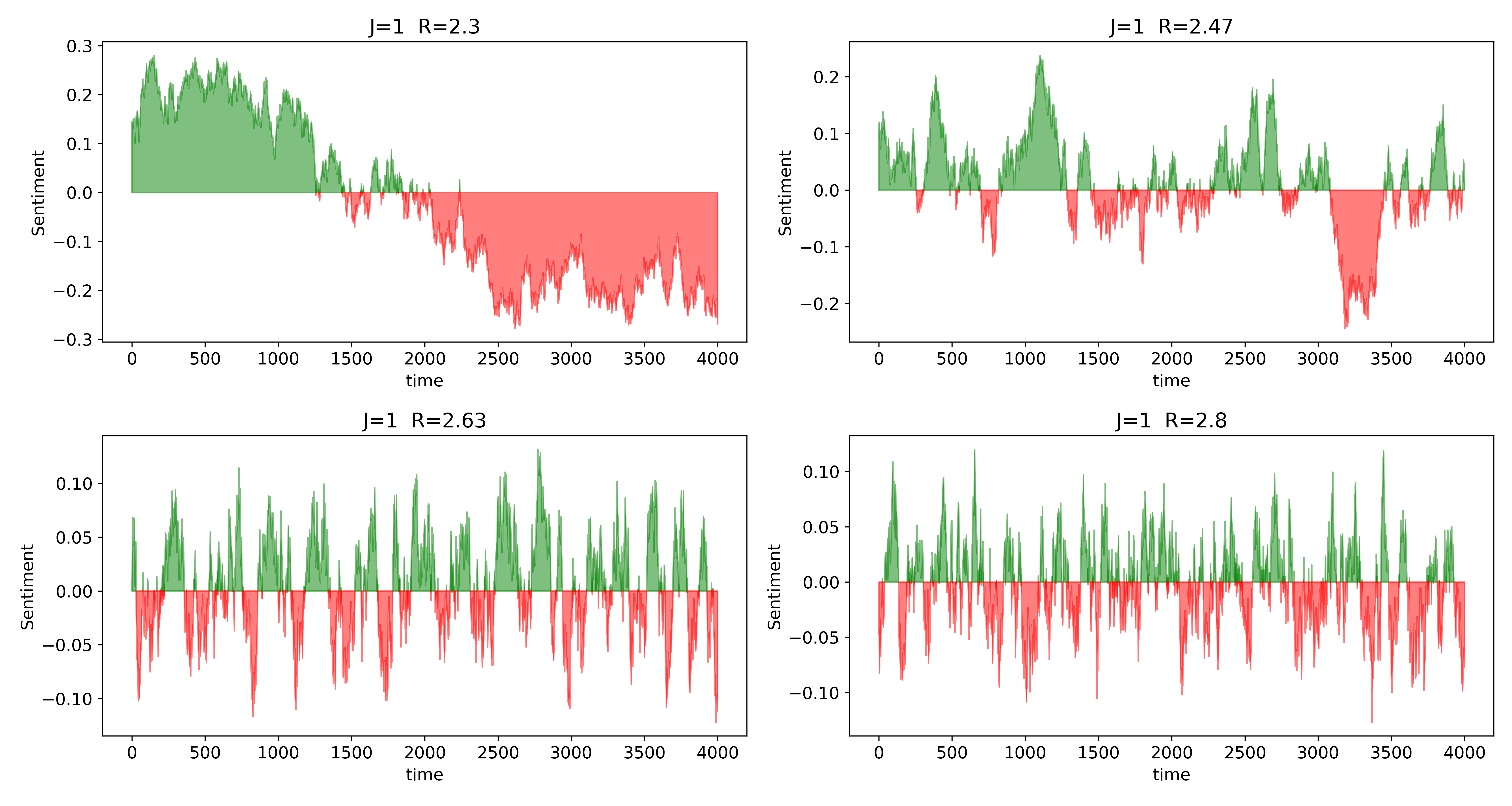
Here we have plotted the net sentiment of the market which we will call <\(S(J,R)\)> as function of \(R\) for a given \(J=1\). Our simple and idealistic indeed shows some very exciting results. First we see that this is very similar to actual return of a market. Second, we see an interesting trend as a function of \(R\) in this artificial market. For small \(R\), we see that the market sentiment is rather robust and the “herd behavior” is maintained. Meaning, once the market is in a state of “bull” or “bear”, it continues on that state for a while till a peaking stimulus is reached. This is contrasting to the big \(R\) case where the market is quite rabidly fluctuating with sentiments. This is indeed true in reality too. For instance, a small \(R\) limit would correspond to what analysts usually call Macro, or essentially the long time dynamics. For long term inverters, who buy-sell stocks once a year or once a month, their “sentiment” is seldom affected by coupling of their stocks to other sectors, they are indeed called “value/growth” investors. While day traders, are greatly affected by everyday news (for example, a sudden drop in oil prices would influence gold/bond market for day traders). Thus it is easy to see that the the longer we are waiting in the market, smaller the \(R\) is in our model and shorter we trade, larger \(R\) is. To make it clearer, lets look at monthly, weekly, daily return of a typical stock - AAPL

This clearly shows that as the investment time increases, the stocks get more stochastic just like our model.
Now, for a non physics mind, this whole idea of modeling the above way, stems from a physics concept called Ising model. Physicists use this same model to study the dynamics/evolution of spins in a lattice which leads to magnetism and indeed \(H\) is called the Hamiltonian of the system. Every system in physics is modeled by writing a physical/experimental motivated \(H\) that you think the system would try to minimize and then use it to predict and infer things about the system. This same model is also used by chemists and material scientists to study how binary alloys order where instead of spin/market sentiment, every site can either have compound A or B. And infact \(R\) is the temperature of the given system.
Now one can add more complications to the model by relaxing a wide range of approximations like change \(J\) to \(J_{ij}\) to be position dependent and much more. There is indeed lot to decipher from this simple system which we will save it for another blog. But the idea illustrated here is the philosophy of physics-To model systems using physical motivations using the beautiful language of math. These are not mere toy models and more sophisticated math models are used in wall streets to make big $.
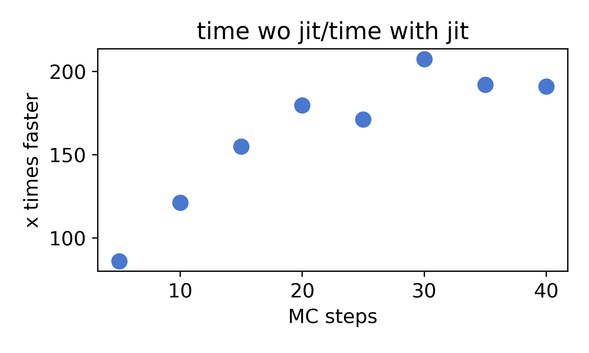
Finally the point of this blog was to see how numba performs, to see that we rewrite the same code without the @jit command and run the following test with respect to number of time steps
time_jit=[]
steps=[5,10,15,20,25,30,35,40]
for j in steps:
    a=%timeit -n1 -r1 -o -q for i in range(10):E=calculate(T=j,N=36,eqSteps=1,mcSteps=j,J=J)
    time_jit.append(a.best)
time_nojit=[]
for j in steps:
    a=%timeit -n1 -r1 -o -q for i in range(10):E=calculate_nojit(T=j,N=36,eqSteps=1,mcSteps=j,J=J)
    time_nojit.append(a.best)
fig,ax=plt.subplots(figsize=(5,3))
ax.scatter(steps,[time_nojit[i]/time_jit[i] for i in range(len(time_jit))],s=80)
ax.set_xlabel("MC steps")
ax.set_ylabel("x times faster")
ax.set_title("time wo numba/time with numba")
plt.tight_layout()
plt.savefig("jitvnojit.png",dpi=400)
plt.show()
and Viola !

We almost have 200 times increase in speed and without numba, it is almost impossible to run more than \(10^{3-4}\) runs in a everyday laptop. Well now I have some data to show to my prof. Until next time.
PS: there are lot more interesting things to be shown/done with this same model and we shall do it in the next session and also explain the idea of “emergence” in physics and how it is beautifully mapped to the market
Topics to explore
physics coding topology python perovskite numba Monte-carlo Julia tight-binding talk susceptibility spin-waves quantum quamtum pysktb optimization finance field-theory advisor Superconductivity Slaster-koster Quantum QFT Physics BdG