After a conference hosted by AFOSR (Air Force Office of Science and Research), I met with an interesting bloke who introduced me to this new language called Julia, that is as fast as FORTRAN/C and yet quick and easy to prototype as Python. Though it was tempting, I brushed off that idea that it could be really worthwhile trying until I met with a snag in one of my research projects.

Short Introduction to the Perovskite Problem

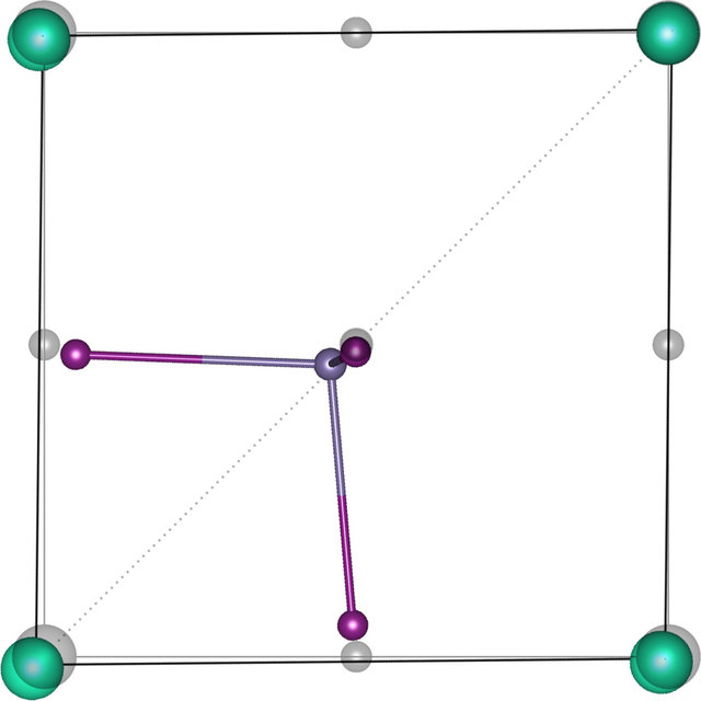
Here’s the deal, we had this very intriguing idea that in Hallide perovskites, the structures can be mapped to a pseudo classical spin vector. Details of which are published in this article [1]. To give a gist, Hallide perovskites are systems that have the formula $ABX_3$ where the $B$ atom is surrounded by 6 $X$ atoms giving it a local octahedral symmetry. In the article we showed that the system undergoes a ferroelectric transition which pushes the central atom $B$ towards body diagonal reducing the local symmetry from “octahedral” to “tetrahedral” forming $BX_3$ tetrahedron units. Here’s the picture of that

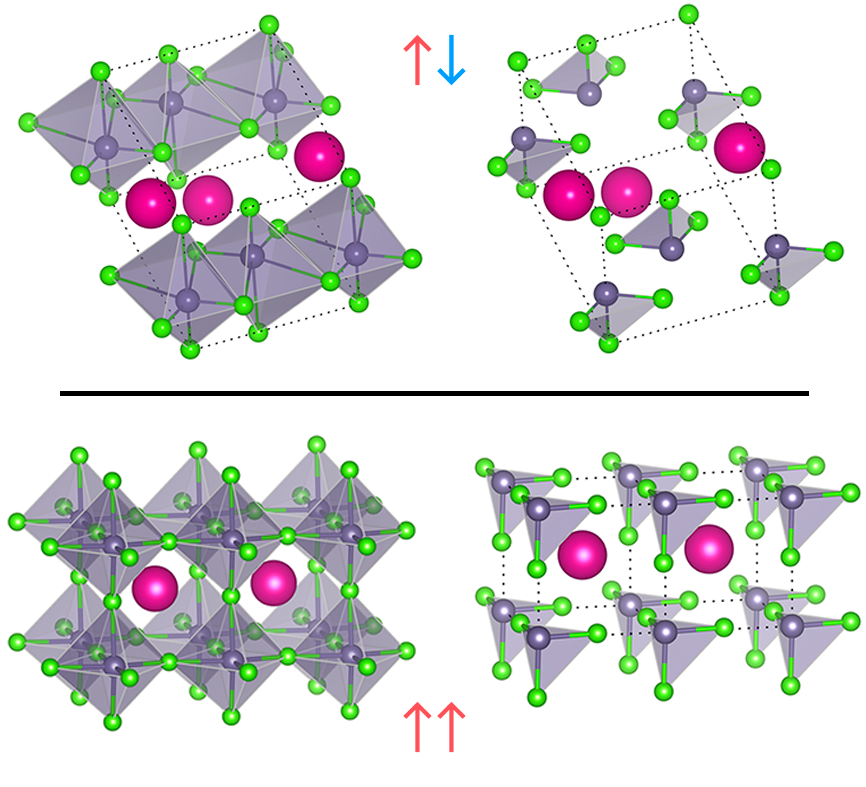
This is taken from yet another old paper [2] where we showed why and how this happens. The resulting effect of this is that the singular units of tetrahedrons, now contain a cloud of electron density that sticks at the tail giving the tetrahedral unit a net dipole charge point in the $(1,1,1)$ body diagonal direction. In the next paper [1], we came up with a clever way of relating this structure to another polymorph structure that is in monoclinic structure. We realized that the mono-clinic structure is actually the same system with the tetrahedrons pointing in opposite direction as shown bellow. Thus if one considers the orientation of the tetraehedron/dipole as a classical pseudo spin vector in real space, the Ferromagnetic arrangement of the system is the perovskite structure while the Antiferromagenetic arrangement is the monoclinic. And it turns out that along with the electric dipole interaction, the system also can stabilize itself by delocalizing its electrons by being in a octahedral environment where one has more periodic chains of atoms, thus reducing the potential energy (or) another way to understand this is to see that being in octahedral environment allows for more “bond” formation and thus reduces the total energy of the system ( we will cover a separate blog post of why bond formation reduces the energy)

This way of looking at these two structures gives very important insights to their stability and why they are shaped the way they are. The perovskite form of this system is a very promising candidate for Solar cell with one of the highest efficiency, but the problem being it degrades to form other structures. If one could understand what stabilizes the crystal in the given structure, we could in principle control the degradation. Secondly, because of the difference in band gap of the monoclinic and perovskite system, If one could transition back and forth between them, one could have a opaque material to a transparent material that is a solar cell. This might be possible say with electric field as the pseudo spins are nothing but dipoles in space.

Okay, so having said all these, the goal for future (read current) work was to predict if such transitions could be realized and if so, how much of an electric field or Temperature difference does one need to do that. A viable approach for this would be to write down the spin Hamiltonian and derive a susuptablity tensor. The Hamiltonian for this system when one considers only a up and down orientation of the pseudo spins turns out to be

Where $\mathcal{g}$ is the coupling constant. This some-what brutal expression can still be solved and shown to have the perovskite and monoclinic as ground state solution based on the sign of $\mathcal{g}$. For a generic spin orientation, it turns out that $H_{d i p o l e}$ remains almost the same ( its just the dipole-dipole classical interaction ) but $H_{b o n d}$ is more sophisticated that a fairly in-adept theorist like myself is unable to decipher. So we turn out to approximating it and making it tractable. On close inspection, it seems natural that the bond formation of the central atom $B$ can be approximated to linear order to the number of nearest $X$. This is brilliant, because we can now numerically compute $H_{b o n d}$ as $\sum^6_{i}r_i$ where $r_i$ is the nearest neighbor distance (NND) to the 6 $X$ atoms surrounding $B$ for different orientation of $BX_3$ tetrahedrons. Thus we now have all the ingredients for solving the complete Hamiltonian which is given by

where

and $U(\theta_1,\phi_1,\theta_2,\phi_2)$ is known numerically. We now can solve \ref{eq:2} using Monte-carlo technique where we sample new orientation of the spins and calculate the NND for estimating $U$ and analytically solve $H_{d i p}$ and proceed to next step. This also helps us couple electric field to the calculation as it is, but another term added that couple spins of particular direction ! But the snag here is that NND algorithms are computational expensive. For instance the in python, the most efficient one written using cython costs around .09 sec for single calculation of a $5x5x5$ super cell. And this is where Julia comes in, speeding things up.

Getting hands dirty with Julia

I am going to outline a quick prototype of the code to calculate the total energy I wrote in Julia (remember this might still be amateur as I have been playing around with Julia just for a week and thought this QMC project might be a good introduction).

We start by importing the required packages, we also use the pymatgen module in python created by MaterialsProject to easily read and import structure data.

using LinearAlgebra
using StaticArrays
using PyCall
using Plots
using Distances
using Statistics
theme(:dark)
using PlotlyJS
p = pyimport("pymatgen")

The idea behind Julia is to define types just like in case of C which then is stored as custom data types at machine level which utilizes the full power of low level types likle Int64 and Float64. For us, we create a type called tetra which holds the positions of the 3 $X$ atoms (which is Cl in this example) and 1 $B$ atom (which is Ge)

struct tetra
    ge::Array{Float64,1}
    cl1::Array{Float64,1}
    cl2::Array{Float64,1}
    cl3::Array{Float64,1}
end 

We then write a function that takes a set of 3D coordinate and rotates it in 3D space that is anchored at anc by an angle theta with respect to axis. For a given tetrahedron, we will rotate it with respect to the center of mass of the tetrahedron which is $\sum_{i=1}^4 \frac{r_i}{4}$ of the tetrahedron vertex.

icross(b) = copy(Transpose(hcat([cross(Matrix(1.0I, 3, 3)[:,i],b) for i in 1:3]...)));
anchor(tetra) = (tetra.ge+tetra.cl1+tetra.cl2+tetra.cl3)/4
function Mdot(a1,a2)
    #=redefing dot product like numpy for matrix=#
    a1_1=copy(Transpose(a1))'
    return [dot(a1_1[i,:],a2) for i in 1:3]
end
function rot(coords,anc,axis,theta)
    #=rotate coords by theta wrt anc with axis as axis=#
    theta %= 2 * pi
    rm=exp(icross(axis/norm(axis))*theta)
    val=Mdot(rm,(coords-anc))+anc
    return val
    end;

function rot_tetra_test_1(t::tetra,axis::Array{Float64,1},theta)
    #=rotate all atoms in tetra by theta with axis = axis=#
    anc=anchor(t)
    ge=rot(t.ge,anc,axis,theta)
    cl1=rot(t.cl1,anc,axis,theta)
    cl2=rot(t.cl2,anc,axis,theta)
    cl3=rot(t.cl3,anc,axis,theta)
    return tetra(ge,cl1,cl2,cl3)
    end;

Finally function rot_tetra_test_1 takes the tetra structure and rotates it by given theta along axis. Note that unlike python, we here define the type of each variable. This is strictly not needed, but is often a good habit to follow as it helps speed up computation times at times and certainly helps debugging. To test the speed at which this works, we create a $5x5x5$ system and rotate every tetrahedron

@time begin
n=5
system=Array{tetra,3}(undef,n,n,n);
for i in 1:length(system)
    system[i]=tetra(randn(3),randn(3),randn(3),randn(3))
    end;

axis=[0,1,1.]
theta=pi/2
for i in 1:length(system)
    system[i]=rot_tetra_test_1(system[i],axis,theta)
	end;
end

we get the following output

Wait what ! 2.8 seconds for just rotating ? Well, this is so because the first run involves compiling all the functions and structures and hence the down time. Running it again, we see that it actually is

which is the reason we now use julia. The speed of computing 125 flips amounts to around $5\mu s$ adding a bunch of over head for other calculation, this would amount to around $20000$ flips a second. Which is indeed a nice count. All this in my Macbook Pro ‘18. Running in a cluster, this would complete a full MC calculation in an hour or so.

Now the heavy lifting comes for calculating the NN distance, forfeiting the complex algorithm, we will look at the nearest cell of tetra in all 3 directions and create a distance matrix between the central $B$ atom and all $X$ atoms from nearest cells. To do this, comes the interesting part, what should we do about the edge atoms? well we impose periodic boundary conditions and study the system as function of $n$ (system size) and hope that it converges w.r.t to that.

function get_nn_1(system,pos,size)
    #= Get first 6 Nearest neibghors to Ge atoms 
    which are Chlorine with PBC=#
    a=(-system[1,1,1].ge+system[1,1,2].ge)[3]
    function pbc(i,n) 
        if i>n
            return i-n,a*size
        elseif i<=0
            return n,-a*(size-1)
        else 
            return i,0
        end
    end
    tmp=Array{Float64, 1}[]
    for i in -1:1
        for j in -1:1
            for k in -1:1
                i1,ai=pbc(pos[1]+i,size)
                j1,aj=pbc(pos[2]+j,size)
                k1,ak=pbc(pos[3]+k,size)
                push!(tmp,system[i1,j1,k1].cl1+[ai,aj,ak])
                push!(tmp,system[i1,j1,k1].cl2+[ai,aj,ak])
                push!(tmp,system[i1,j1,k1].cl3+[ai,aj,ak])
            end
        end
    end
    return tmp
end

Finally, we get calculate $U$ by calculating the distance and taking either the mean or variance of the closest 6 NN $X$ atoms

function get_mean_var(system,pos,return_type="var")
    #= Get the mean or variance of a 
    position of lattice  wrt bond distance=#
    sys=system[pos[1],pos[2],pos[3]]
    distance_1=colwise(Euclidean(), sys.ge, copy(hcat(get_nn_1(system,pos,n)...)))
    nn=sort(distance_1)[1:6]
    var_sys=var(nn)
    mean_sys=mean(nn)
    if return_type=="mean"
        return mean_sys
    else
        return var_sys
    end
end

To test it out, lets first load up the system, which is a 3D matrix holding tetra structure with real numbers from a perovskite system CsSiI$_2$ using pymatgen (Yes you can import python modules in Julia ! yay !)

 function make_symstem(n=2)
    cssii2=p.Structure.from_file("Cssii2.cif")
    struc1=cssii2.copy()
    struc1.make_supercell([[n,0,0],[0,n,0],[0,0,n]])
    dist=cssii2.get_distance(1,3)+.1
    positions=Array{Int64, 1}[]
    for i in struc1
        if i.species_string=="Si"
            push!(positions,struc1.get_neighbor_list(dist,[i])[2])
        end
    end
    system=Array{tetra,3}(undef,n,n,n);
    cnt=1
    for i in 1:n
        for j in 1:n
            for k in 1:n
                ge=get(struc1,reverse(positions[cnt])[1]).coords
                cl1=get(struc1,reverse(positions[cnt])[2]).coords
                cl2=get(struc1,reverse(positions[cnt])[3]).coords
                cl3=get(struc1,reverse(positions[cnt])[4]).coords
                system[i,j,k]=tetra(ge,cl1,cl2,cl3)    
                cnt+=1
            end
        end
    end
    return system
end

n=4
system=make_symstem(n);

Then we take a single tetrahedron at the $(4,4,2)$ site and then rotate it along $\theta=(1,1,1)$ and $\phi=(1,0,0)$ axis in small steps from $(0,2\pi)$ and then plot $U(\theta,\phi)$

a=[]
nk=100
@time begin
for i in LinRange(0, pi*2, nk)
        for j in LinRange(0, pi*2, nk)
			theta=i
			axis=[2,2,2.]
			system_test=copy(system)
			pos_1=[4,4,2]
			system_test[pos_1[1],pos_1[3],pos_1[3]]=
			        rot_tetra_test_1(system[pos_1[1],pos_1[3],pos_1[3]],axis,theta);
			theta=j
			axis=[1,0,0.]
			system_test[pos_1[1],pos_1[3],pos_1[3]]=
			        rot_tetra_test_1(system_test[pos_1[1],pos_1[3],pos_1[3]],axis,theta);
			            
			mean_1=mean([get_mean_var(system_test,[i,j,k],"var") for i in 1:n for j in 1:n for k in 1:n])
			push!(a,mean_1)
			end
end
end

This entire $100x100=10^4$ calculations took $4s$ to run. We can plot it using

a=reshape(a,nk,nk)
contourf(LinRange(0, pi*2, nk),
    LinRange(0, pi*2, nk), a,levels=10,aspect_ratio = 1)

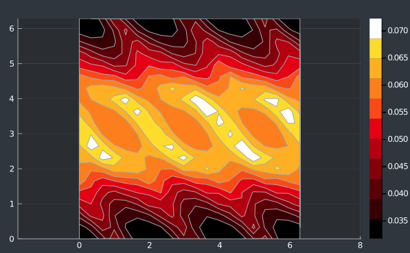
which gives us

We can see that at $\thea=\phi=0$ the minimum U occurs which is the lowest energy and the system has a nice periodicity. Well this verifies at least to some level that the code is working.

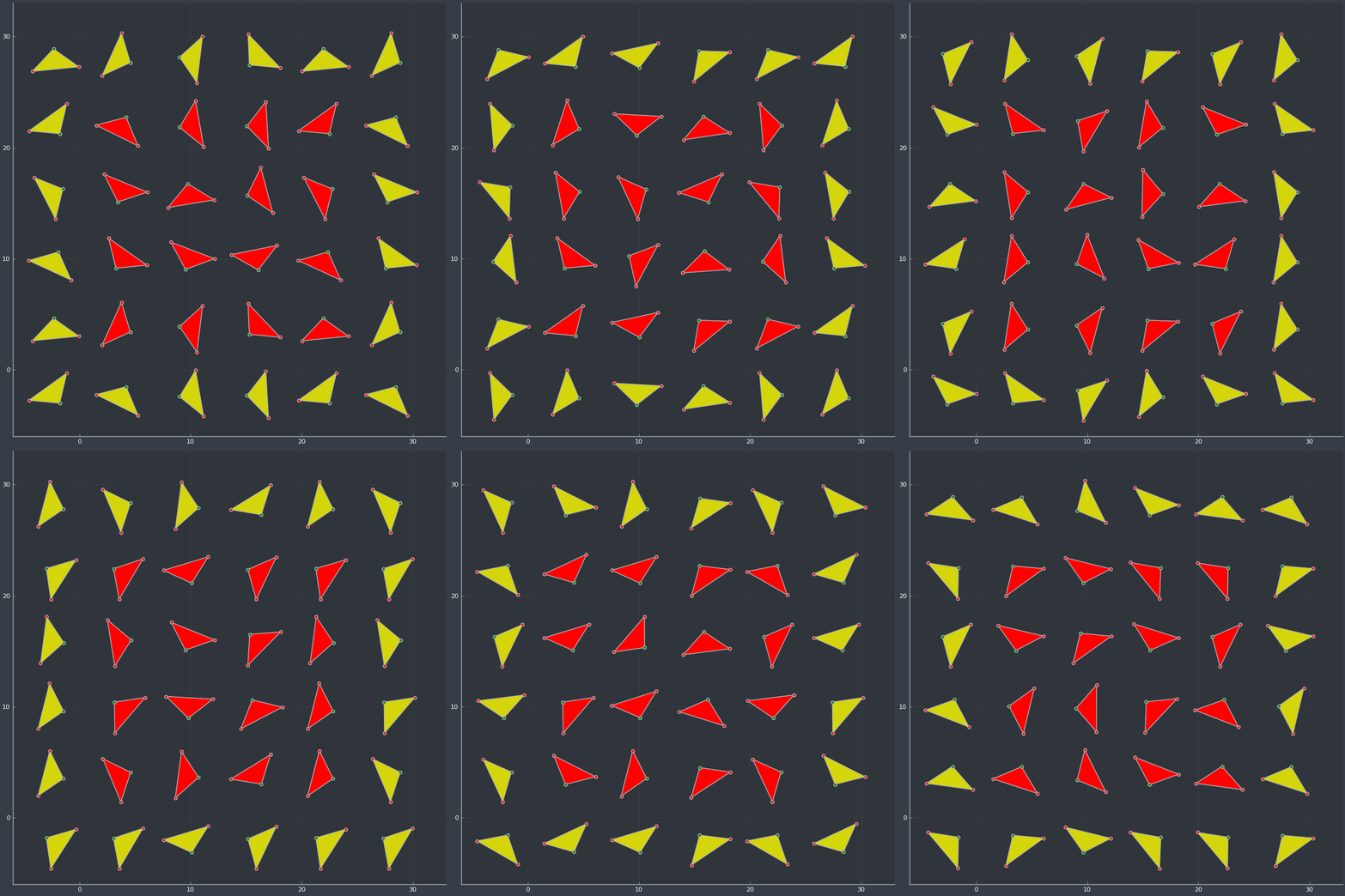
Now finally before we leave, lets do a final check to see that the system is indeed what it is and periodicity and rotation is maintained. For this, we plot the tetrahedrons (or their projection) along the $x-y$ axis and randomly rotate each units by random angle along $(0,0,1)$ axis ($z$-axis). We will plot their periodic counter part in different color just to make sure that rotating an edge atom has effect on the other side because of periodic boundary condition. We do that by

system_test=copy(system)
function plot_perov()
    plt=plot(5,xlim=(-6,33),ylim=(-6,33), aspect_ratio=1,legend=false,size = (800, 800))
    global system_test
    pos_1=[rand(1:4),rand(1:4),1]
    axis=[0,0,1.]
    theta=pi*2*rand()
    system_test[pos_1[1],pos_1[2],pos_1[3]]=
            rot_tetra_test_1(system[pos_1[1],pos_1[2],pos_1[3]],axis,theta);
    for i in 0:n+1
    for j in 0:n+1
        a=(-system[1,1,1].ge+system[1,1,2].ge)[3]
        function pbc(i,n) 
            if i>n
                return i-n,a*n
            elseif i<=0
                return n,-a*(n)
            else 
                return i,0
            end
        end
        i1,ai=pbc(i,n)
        j1,aj=pbc(j,n)
    x=[]
    y=[]
    if ai!=0 || aj !=0
            col="yellow";alpha=0.8
    else 
            col="red";alpha=1
    end
    x=[system_test[i1,j1,1].ge[1]+ai
            ,system_test[i1,j1,1].cl1[1]+ai
            ,system_test[i1,j1,1].cl2[1]+ai
            ,system_test[i1,j1,1].ge[1]+ai]
        
    y=[system_test[i1,j1,1].ge[2]+aj
            ,system_test[i1,j1,1].cl1[2]+aj
            ,system_test[i1,j1,1].cl2[2]+aj
            ,system_test[i1,j1,1].ge[2]+aj]
    plt=plot!(x,y,color="grey",label="")
    plot!(Plots.Shape(x,y),label="",color=col,alpha=alpha)
    scatter!(plt,x[2:3],y[2:3],color="red",label="")
    scatter!(plt,[x[1]],[y[1]],color="green",label="")
    end
end
end

This plots a very beautiful Movie that gives us this

It is easy to see that a change in edge tetrahedrons (or their projected triangle) has an effect on the opposite boundary triangle denoted by yellow atom.

Not bad for a quick 2 day foray into Julia. Will update as soon as I add more modules. Ciao.

Part 2 continued here

Github repo of the project can be found here

References