Continued from previous post that can be found here
So, mid way through the project, I realized that I had written the expression for PBC tiny bit wrong and that lead to disastrous calculation of U value. So in this post, let us rectify that and add Dipole terms to the system.
PBC for a given index, is actually given by (after hours of breaking the nerves in my fried brain)
function pbc_1(system,index)
    eval_1(i,n)= ((abs(i)-1) ÷ n)*((sign(i)+1) ÷ 2) - ((sign(i-1)-1) ÷ 2)*((i-n) ÷ n)
    index_1(i,n)=((abs(i+n-1) % n)+1)
    unit_size=size(system)[1]
    a=(-system[1,1,1].ge+system[1,1,2].ge)[3]*unit_size
    uc=eval_1.(index,unit_size)*a
    index_mod=index_1.(index,unit_size)#index .% (unit_size+1)
    return index_mod,uc
    end;
pbc_1 takes the system (which stores the tetra object in 3D space in a $nxnxn$ matrix) and index to which it needs to calculate the corresponding PBC tetra unit inside the unit cell and also the value to which it needs to be moved by. It turns out because of the dispatch mechanism in Julia, it makes more sense to write a dispatchable function to get the system at a given index with PBC. Using the above pbc_1 one can use something like
#----get the tetra of a system at given index with PBC
function system_at_index(system,index)
    index_mod,uc=pbc_1(system,index)
    tetra_tmp=system[index_mod[1],index_mod[2],index_mod[3]]
    ge=tetra_tmp.ge+uc
    cl1=tetra_tmp.cl1+uc
    cl2=tetra_tmp.cl2+uc
    cl3=tetra_tmp.cl3+uc
    return tetra(ge,cl1,cl2,cl3)
    end;
And thus our NN function previously written, reduces to
# NN algorithm
function get_nn_2(system,pos)
    tmp=Array{Float64, 1}[]
    for i in -1:1
        for j in -1:1
            for k in -1:1
                index_tmp=pos+[i,j,k]
                temp=system_at_index(system,index_tmp)
                push!(tmp,temp.cl1)
                push!(tmp,temp.cl2)
                push!(tmp,temp.cl3)
            end
        end
    end
    return tmp
end
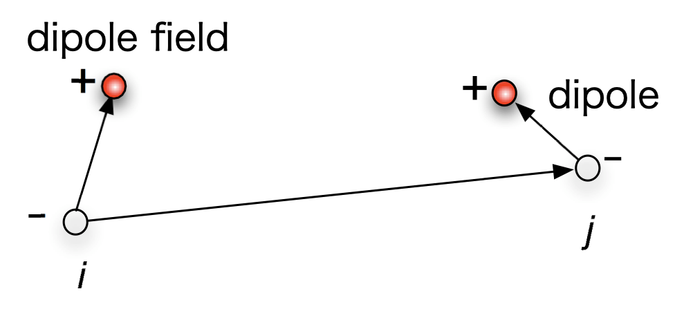
Having corrected this, we can now start writing the dipole equation. For a given set of dipoles as shown bellow,

Dipole interaction energy can be derived and is given by
\[\begin{equation}U_{\mathrm{dd}}=\frac{1}{4 \pi \epsilon_{0} r_{i j}^{3}}\left[\vec{\mu}_{i} \cdot \vec{\mu}_{j}-3 \frac{\left(\vec{\mu}_{i} \cdot \mathbf{r}_{i j}\right)\left(\mathbf{r}_{i j} \cdot \vec{\mu}_{j}\right)}{r_{i j}^{2}}\right]\end{equation} \label{eq:1}\]Where $\mu_{i}$ is the dipole vector and $r_{i j}$ is the vector connecting the dipoles. Here, for the sake of simplicity, we will ignore the pre-factors and code just the form of it. This doesn’t take out any physics as for our case, the strength is arbitrary and infact controlled by the coupling between dipole energy and “bonding” energy.
# Function to get dipole orientation of a tetrahedron
function get_dipol_vec(tetra::tetra)
    return (tetra.ge - (tetra.cl1+tetra.cl2+tetra.cl3)/3)/norm(tetra.ge - (tetra.cl1+tetra.cl2+tetra.cl3)/3)
end


# Get the distance  vector between two tetrahedrons supplying pl will plot it in pl
function get_dipole_dist(tetra1::tetra,tetra2::tetra,pl=nothing)
    r1=(tetra1.ge+tetra1.cl1+tetra1.cl2+tetra1.cl3)/4
    r2=(tetra2.ge+tetra2.cl1+tetra2.cl2+tetra2.cl3)/4
    if pl == nothing
        return r1-r2
    else
        plot_tetra(tetra1,pl)
        plot_tetra(tetra2,pl)
        plot!(pl,[i[1] for i in [r1,r2]],[i[2] for i in [r1,r2]],[i[3] for i in [r1,r2]],color="red",linewidth=3,label="connecting vector r12")
        end;
    end;
Above code get_dipol_vec calculates the dipole vector orientation for a given tetrahedron which is nothing but the distance of $B$ atom to the center of the triangle formed by 3 $X$ atoms. get_dipole_dist calculates the vector connecting the two centers of the tetrahedrons.
function get_dipole_energy_between_tetra(tetra1::tetra,tetra2::tetra)
    r12=get_dipole_dist(tetra1,tetra2)
    r12=r12
    d1=get_dipol_vec(tetra1)
    d2=get_dipol_vec(tetra2)
    four_pe0= 9 * 10^9 #1/4πe0 in N⋅m^2⋅C^−2
    return -dot(d1,d2)+3*(dot(d1,r12)*dot(d2,r12))
    end;
get_dipole_energy_between_tetra implements the \ref{eq:1} formula without the scaling which can be a parameter to be tuned. Now we can actually calculate the change total energy of a single twist of a tetrahedron, which is actually the quantity that determines the acceptance of Monte carlo. For this, we write a function that takes the system, position of the index to make flip and finally axis and theta to rotate the position about. We also need the scaling factor for calculating the two competing energy which is given by
Just to make it easy, we will re-write \ref{eq:2} to $H=\mathcal{g_1} \cdot H_{d i p o l e}+ \mathcal{g_2} \cdot H_{b o n d}$ so that we can check the individual effect while debugging. So now we can calculate the above by
function get_rotation_energy_1(system,g1,g2,pos,axis,theta)
    system_test=copy(system)
    system_test[pos[1],pos[2],pos[3]]=
            rot_tetra_test_1(system_at_index(system,pos),axis,theta);
    nn=[[1,0,0],[-1,0,0],[0,1,0],[0,-1,0],[0,0,1],[0,0,-1]]
    u=0
    for i in nn
        ind,_=pbc_1(system,pos+i)
        u+=(get_mean_var(system_test,ind,"var")-get_mean_var(system,ind,"var"))
    end
    d=get_dipole_energy(system_test,pos)-get_dipole_energy(system,pos)
    return g1*u+g2*d
    end;
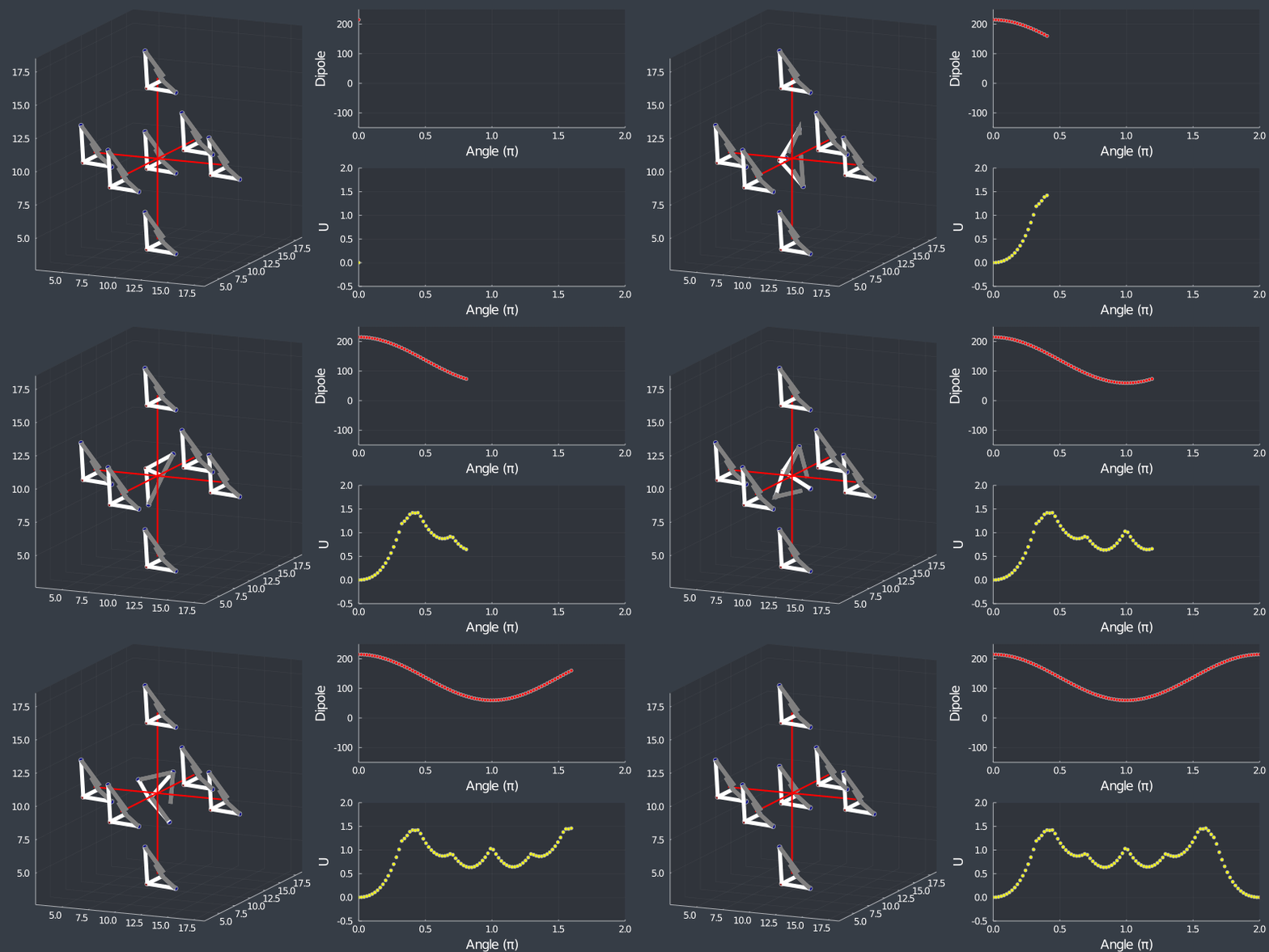
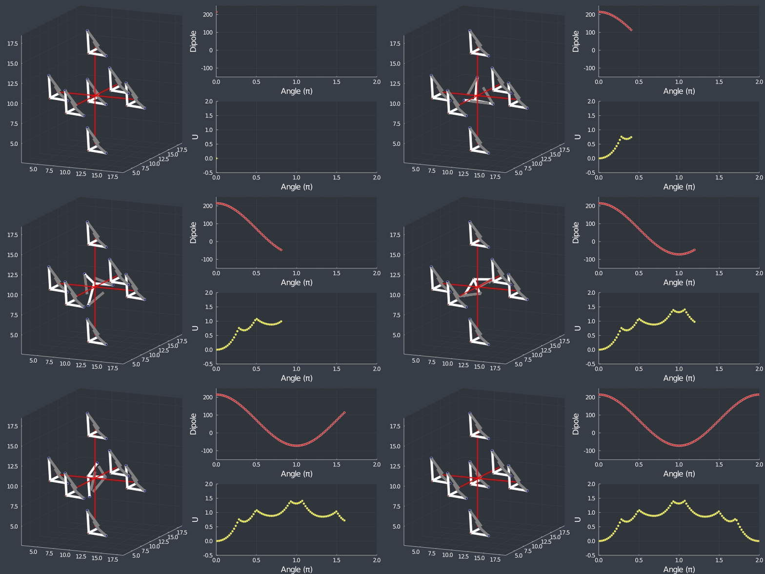
And thus, we have written the entire set of code to calculate the necessary equations. The beauty of Julia is that it is both a lisp language as well as a JIT one, Thus we can plot beautiful objects that are as fast as fortran. So, before leaving lets plot the Dipole energy and U while rotating. Here is the code.
dipole=[]
function rot_draw(i,pl2,pl3)
    pl=plot()#plot(xlim=(-2,10),ylim=(-2,10))
    theta=i
    axis=[1,0,1.]
    system_test=copy(system)
    pos_1=[2,2,2]
    nn=[[1,0,0],[-1,0,0],[0,1,0],[0,-1,0],[0,0,1],[0,0,-1]]
    system_test[pos_1[1],pos_1[2],pos_1[3]]=
            rot_tetra_test_1(system_at_index(system,pos_1),axis,theta);
    tetra1=system_test[pos_1[1],pos_1[2],pos_1[3]]
    plot_tetra(tetra1,pl)
    d=0
    for i in nn
        ge=(tetra1.ge+tetra1.cl1+tetra1.cl2+tetra1.cl3)/4
        pos_new=pos_1+i
        temp=system_at_index(system,pos_new)
        tetra2=(temp.ge+temp.cl1+temp.cl2+temp.cl3)/4
        plot!(pl,[ge[1],tetra2[1]],[ge[2],tetra2[2]],[ge[3],tetra2[3]],color="red",linewidth=2,label="")
        plot_tetra(temp,pl)
        d+=get_dipole_energy_between_tetra(tetra1,temp)
        end;
    scatter!(pl2,[i/(π)],[d],markersize=3,label="",color="red")
    plot(pl,pl2,size = (800, 400),aspect=1)
    u=0
    for i in nn
        ind,_=pbc_1(system,pos_1+i)
        u+=(get_mean_var(system_test,ind,"var")-get_mean_var(system,ind,"var"))
        end;
    l =  @layout([a [b; c]])
    scatter!(pl3,[i/(π)],[u],markersize=3,label="",color="yellow")
    plot(pl,pl2,pl3,size = (800, 400),aspect=1,layout=l)
    end;
Plots.gr()
pl2=plot(size = (800, 800),aspect=1,ylim=(-150,250),xlim=(0,2),xlabel="Angle (π)",ylabel="Dipole")
pl3=plot(size = (800, 300),aspect=1,ylim=(-.5,2),xlim=(0,2),xlabel="Angle (π)",ylabel="U")
anim = @animate for i ∈ LinRange(0,2*pi,100)
    rot_draw(i,pl2,pl3)
end
gif(anim, "animations/complete1_111.gif", fps = 20)
We will do it for various rotation axis


Just as a check, rotating the tetrahedron along the $[111]$ direction, (in which it is oriented at) should not change the dipole, but because of the $C_3$ symmetry of the tetrahedron, one should see a 3 fold symmetry in NN or Bonding energy which is seen bellow !

Next stop, MC…
Github repo of the project can be found here
References
Topics to explore
physics coding topology python perovskite numba Monte-carlo Julia tight-binding talk susceptibility spin-waves quantum quamtum pysktb optimization finance field-theory advisor Superconductivity Slaster-koster Quantum QFT Physics BdG